An Introduction to Stochastic Calculus and Itô's Lemma

I’ve been working on diffusion models since 2022, and that led me to the stochastic calculus behind them. One natural way to understand continuous-time diffusion models is through stochastic differential equations (SDEs)¹. If you learned ordinary calculus first, SDEs can feel unfamiliar at the beginning. This post is my attempt to explain the pieces that helped them click for me before getting into the deeper math behind diffusion SDEs.

When working with SDEs, we deal with stochastic processes $X_t$, random paths that evolve over time. Each run gives a different trajectory. In principle, these processes can run forever ($T=\infty$), so they live in an infinite-dimensional space. Here I’ll keep the setup simple and take $X_t \in \mathbb{R}$. Examples include stock prices, population dynamics, and the pH level of a chemical solution.

We’ll start with why $(dW_t)^2 = dt$ through quadratic variation. Then we’ll build stochastic integrals and Itô’s Lemma, solve a few classic SDEs, and end with Brownian motion on a circle to show how geometry enters the picture.

When we write $\mathbb{E}[X_t]$ or $\mathbb{E}[f(X_t)]$, the expectation is over sample paths. Imagine running the process many times. Each run gives a different random path. The expectation is the average value across those runs. In practice, you can think of simulating 10,000 Brownian motion paths and averaging the quantity of interest over all 10,000 samples.

Quadratic Variation

In regular calculus, when you have an infinitesimal $dx$, the square $(dx)^2$ is so small we ignore it. But Brownian motion $W_t$ is “rough” enough that the following holds

To see where this comes from, start with the definition of quadratic variation and then derive the result.

The quadratic variation of a stochastic process $X_t$ over $[0, T]$ is

where $0 = t_0 < t_1 < \cdots < t_n = T$ is a partition of $[0, T]$ with grids going to zero as $n \to \infty$. For Brownian motion, this limit exists and equals $T$.

To derive this, consider partitioning the interval $[0, T]$ into $n$ equal subintervals with $\Delta t = T/n$. The sum of squared increments is

Each increment $(W_{t_i} - W_{t_{i-1}})$ is Gaussian, that is, $(W_{t_i} - W_{t_{i-1}}) \sim \mathcal{N}(0, \Delta t)$, and increments are independent, meaning the value of $(W_{t_i} - W_{t_{i-1}})$ doesn’t tell you anything about $(W_{t_j} - W_{t_{j-1}})$ for $i \neq j$. This is what makes the process memoryless. Increments at different times don’t know about each other.

For a Gaussian random variable with variance $\Delta t$, the expected squared value equals its variance, so

This holds because the increment has zero mean: $\mathbb{E}[W_{t_i} - W_{t_{i-1}}] = 0$, so $\text{Var}[W_{t_i} - W_{t_{i-1}}] = \mathbb{E}[(W_{t_i} - W_{t_{i-1}})^2] - (\mathbb{E}[W_{t_i} - W_{t_{i-1}}])^2 = \mathbb{E}[(W_{t_i} - W_{t_{i-1}})^2]$.

So the expected value of the entire sum is

This means the quadratic variation fluctuates around $T$ such that

For a squared Gaussian $Z^2$ where $Z \sim \mathcal{N}(0, \sigma^2)$, we have $\text{Var}[Z^2] = 2\sigma^4$.

Why? Using the rule $\text{Var}[X^2] = \mathbb{E}[X^4] - (\mathbb{E}[X^2])^2$. For a centered Gaussian, $\mathbb{E}[Z^2] = \sigma^2$ and $\mathbb{E}[Z^4] = 3\sigma^4$ (the fourth moment), so $\text{Var}[Z^2] = 3\sigma^4 - (\sigma^2)^2 = 2\sigma^4$.

Therefore

Since the increments are independent, the variance of the sum is

As we make the partition finer, the randomness washes out and the sum approaches $T$. The sum of squared increments becomes more predictable, not less. This is the quadratic variation of Brownian motion. It stays non-zero and becomes deterministic in the limit.

Since the quadratic variation over $[0, T]$ equals $T$, the quadratic variation over any infinitesimal interval $[t, t+dt]$ equals $dt$. In differential form, this gives us equation (1)

This is what makes stochastic calculus different from regular calculus. When we later do Taylor expansions and decide which second-order terms to keep, we can’t ignore $(dW_t)^2$ because it equals $dt$, not zero.

We can also express the quadratic variation as an integral. Taking the limit of the discrete sum

In other words, the “integral” of $(dW_t)^2$ over time is just ordinary integration of $dt$.

For more detail, Øksendal’s book² (Chapter 3) and Gardiner³ (Chapter 4.2) work through the full argument.

Random Fluctuations through Brownian Motion

Brownian motion $W_t$ is our fundamental noise source. Think of it as a continuous random walk. It starts at zero ($W_0 = 0$), and each increment $W_t - W_s$ is Gaussian with variance $t - s$. Importantly, increments at different times are independent: the past doesn’t influence the future.

The simplest SDE is pure Brownian motion: $dX_t = dW_t$. Here a particle changes position randomly at each instant, with no drift term, only noise. The simulation below shows what those paths look like:

import numpy as np
import matplotlib.pyplot as plt

np.random.seed(42)
T, n_steps, n_paths = 1.0, 500, 5
dt = T / n_steps
t = np.linspace(0, T, n_steps + 1)

# Brownian motion: cumulative sum of Gaussian increments
dW = np.sqrt(dt) * np.random.randn(n_paths, n_steps)
W = np.zeros((n_paths, n_steps + 1))
W[:, 1:] = np.cumsum(dW, axis=1)

plt.figure(figsize=(8, 4))
for i in range(n_paths):
    plt.plot(t, W[i], alpha=0.8)
plt.xlabel('t'); plt.ylabel('$X_t$')
plt.title('Sample Brownian Motion Paths')
plt.show()

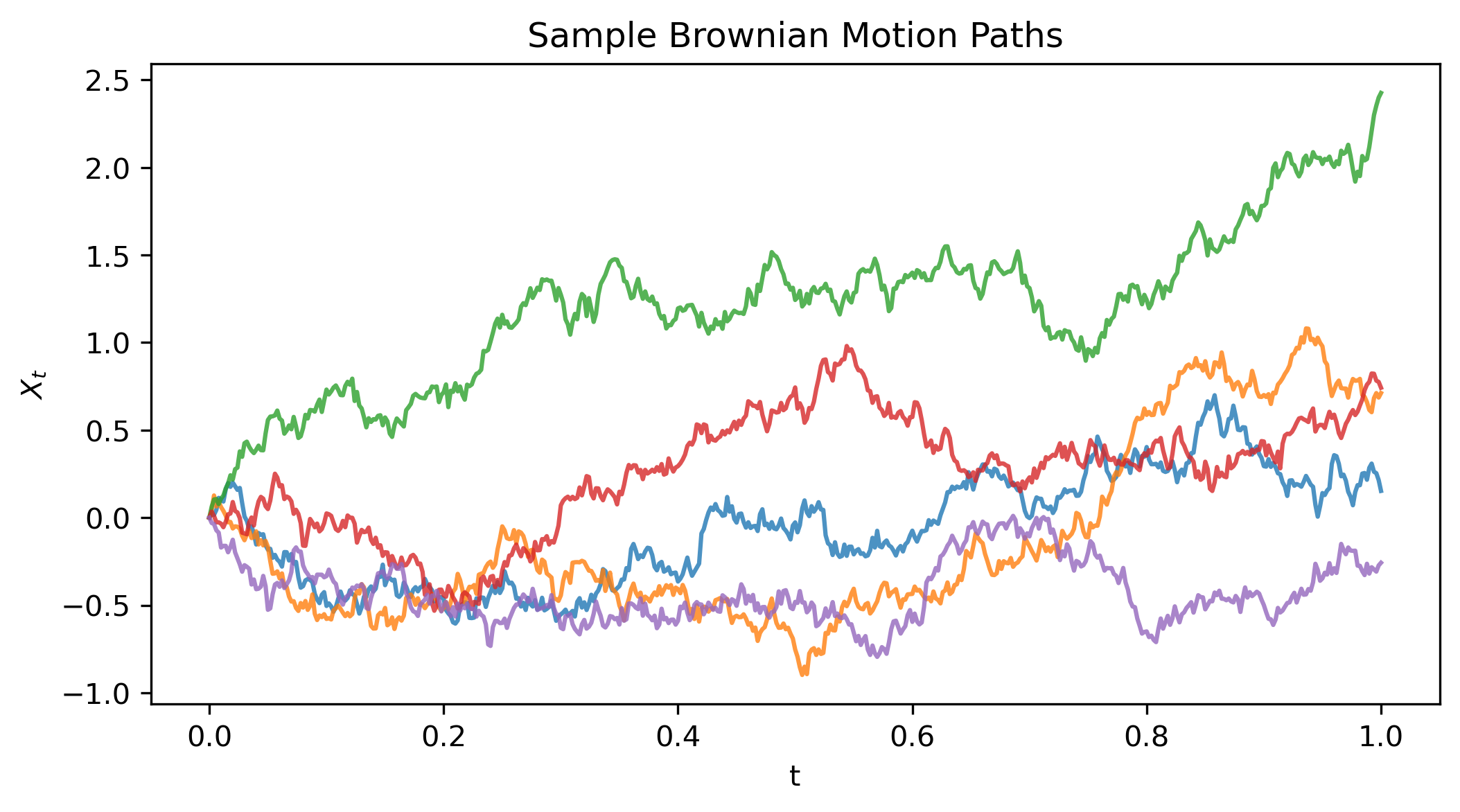Figure 1: Sample Brownian motion paths starting from zero, each taking a different random trajectory.

Each path starts at zero and moves randomly: some drift up, others down. The important point: increments dW = np.sqrt(dt) * randn() have variance dt, which is why $(dW)^2 \sim dt$.

Stochastic Integrals

Before we can solve SDEs, we need to understand stochastic integrals. Unlike ordinary integrals where you integrate with respect to $dt$, here we integrate with respect to Brownian motion $dW_t$. Think of it as multiplying a function by random noise and summing up the results over time. Remember those random paths from Figure 1? Stochastic integrals are built from exactly those Brownian increments.

A simple case is $\int_0^t dW_s$.

Since $W_t$ is the integral of its own differential, we have

since $W_0 = 0$. Think of it as the position of a particle undergoing Brownian motion (like the paths shown in Figure 1) at any time $t$.

This is just the fundamental theorem of calculus: integrating the differential gives you back the function. Same as $\int_0^t ds = t$, but now with randomness.

More generally, for a deterministic function $g(t)$, the Itô integral is

This is defined as the limit of Riemann-like sums: partition $[0, t]$ into small intervals and approximate

Notice we evaluate $g$ at the left endpoint $t_{i-1}$ as this is the Itô convention. As the partition gets finer, this sum converges to the stochastic integral.

Two properties matter here. First, the integral $\int_0^t g(s) \, dW_s$ is a random variable because it depends on which Brownian path you get. Second, it has mean zero: $\mathbb{E}\left[\int_0^t g(s) \, dW_s\right] = 0$. As before, the expectation averages over many Brownian paths.

Why mean zero? Remember the integral is built from the sum $\sum_i g(t_{i-1})(W_{t_i} - W_{t_{i-1}})$. Each Brownian increment has zero mean: $\mathbb{E}[W_{t_i} - W_{t_{i-1}}] = 0$. Since $g(t_{i-1})$ is deterministic (known at the previous time step), we have $\mathbb{E}[g(t_{i-1})(W_{t_i} - W_{t_{i-1}})] = g(t_{i-1}) \mathbb{E}[W_{t_i} - W_{t_{i-1}}] = g(t_{i-1}) \cdot 0 = 0$. The expected value of the sum is zero, so the integral has mean zero.

• Its variance is given by the Itô isometry

What does Itô isometry mean? It tells you how variance accumulates over time. When $g(s)$ is large at some moment $s$, the noise gets amplified there, contributing more to the total variance. The formula is elegant: variance of the stochastic integral = ordinary time integral of $g(s)^2$.

This formula appears in many applications, like computing variances of stochastic processes, proving that numerical methods like Euler-Maruyama converge, or finding stationary distributions (as we’ll do later for the Ornstein-Uhlenbeck process).

For $\int_0^t s \, dW_s$, equation (2) gives variance $= \int_0^t s^2 \, ds = \frac{t^3}{3}$.

We can check the Itô isometry numerically with two choices of $g(s)$: $1$ and $s$. We’ll simulate 10,000 Brownian paths until time $T=1$, compute the stochastic integral for each path, and compare the empirical mean and variance with the theoretical results from Itô isometry.

import numpy as np
import matplotlib.pyplot as plt

np.random.seed(42)
T = 1.0
n_steps = 500
n_paths = 10000
dt = T / n_steps
t_grid = np.linspace(0, T, n_steps)

# Generate Brownian motion paths
dW = np.sqrt(dt) * np.random.randn(n_paths, n_steps)
W = np.cumsum(dW, axis=1)

# Case 1: g(s) = 1
# The stochastic integral is simply W_T
integral_constant = W[:, -1]
var_constant = T

# Case 2: g(s) = s
# Using left-endpoint approximation: sum of g(t_{i-1}) * dW_i
integral_linear = np.zeros(n_paths)
for i in range(n_steps):
    g_value = t_grid[i]  # g(s) = s evaluated at left endpoint
    integral_linear += g_value * dW[:, i]
var_linear = T**3 / 3

# Create side-by-side plots
fig, axes = plt.subplots(1, 2, figsize=(14, 5))

# Plot 1: g(s) = 1
axes[0].hist(integral_constant, bins=50, density=True, alpha=0.7, 
             label=f'Simulated (mean={np.mean(integral_constant):.3f}, var={np.var(integral_constant):.3f})')
x1 = np.linspace(-4, 4, 100)
axes[0].plot(x1, 1/np.sqrt(2*np.pi*var_constant) * np.exp(-x1**2/(2*var_constant)), 
            'r-', linewidth=2, label=f'Theory: $\mathcal(0, {var_constant:.3f})$')
axes[0].set_xlabel(r'$\int_0^T dW_s = W_T$')
axes[0].set_ylabel('Probability Density')
axes[0].set_title('$g(s) = 1$ (constant)')
axes[0].legend()
axes[0].grid(alpha=0.3)

# Plot 2: g(s) = s
axes[1].hist(integral_linear, bins=50, density=True, alpha=0.7, 
             label=f'Simulated (mean={np.mean(integral_linear):.3f}, var={np.var(integral_linear):.3f})')
std_linear = np.sqrt(var_linear)
x2 = np.linspace(-3*std_linear, 3*std_linear, 100)
axes[1].plot(x2, 1/np.sqrt(2*np.pi*var_linear) * np.exp(-x2**2/(2*var_linear)), 
            'r-', linewidth=2, label=f'Theory: $\mathcal(0, {var_linear:.3f})$')
axes[1].set_xlabel(r'$\int_0^T s \, dW_s$')
axes[1].set_ylabel('Probability Density')
axes[1].set_title('$g(s) = s$ (linear)')
axes[1].legend()
axes[1].grid(alpha=0.3)

plt.suptitle('Stochastic Integral Distributions for Different Functions $g(s)$', 
             fontsize=14, y=1.02)
plt.tight_layout()
plt.show()

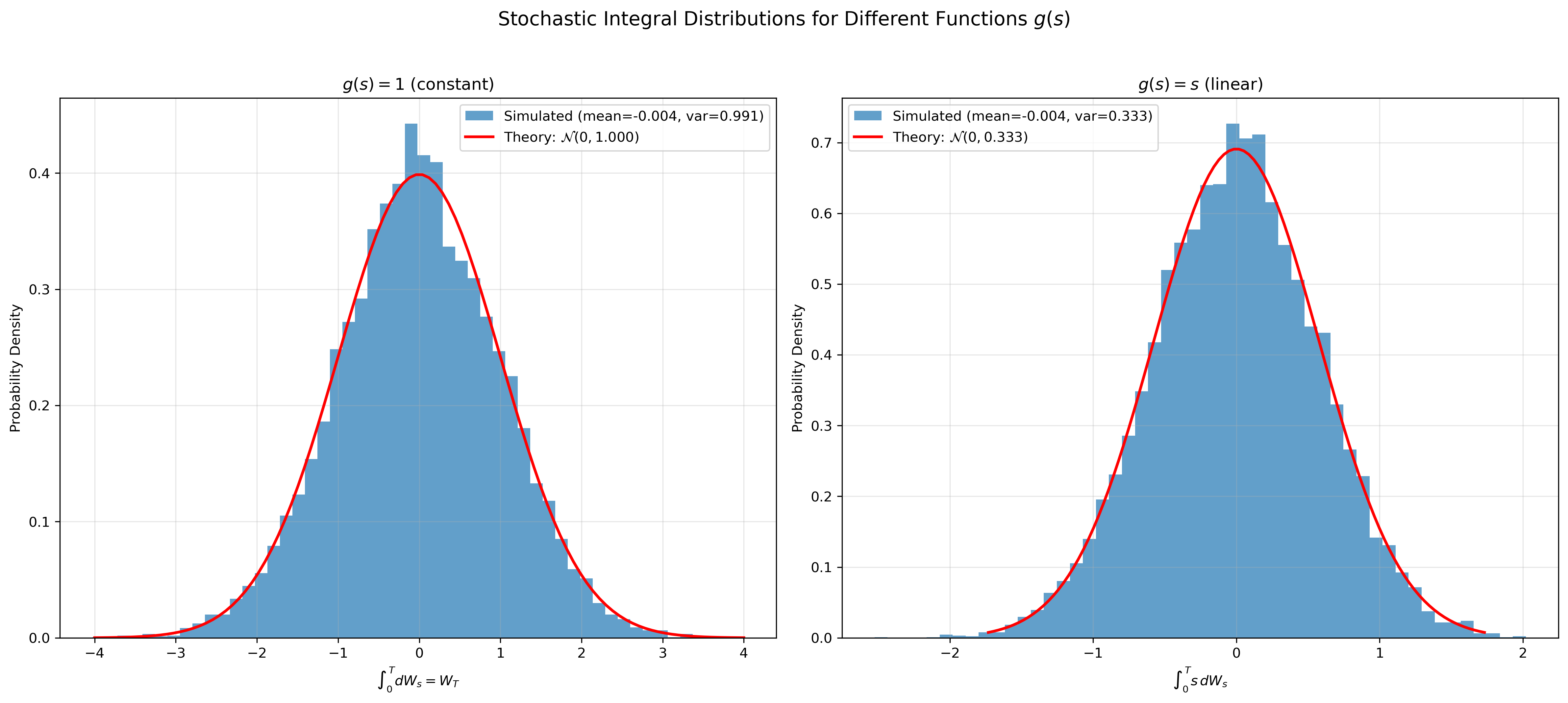Figure 2: Distribution of stochastic integrals for two different functions: $g(s)=1$ (left) and $g(s)=s$ (right). Both are Gaussian with different variances.

The simulation confirms the Itô isometry: we computed 10,000 stochastic integrals (one for each sample path). Each individual integral $\int_0^T g(s) \, dW_s$ is a random variable. The histograms show the distribution of these random variables across all paths. For $g(s) = 1$, the empirical variance matches the theoretical prediction $T = 1$ and for $g(s) = s$, variance = $T^3/3 \approx 0.333$. Notice how the linear function produces a narrower distribution since its variance is smaller.

Wait, the distributions look Gaussian, right? The stochastic integral $\int_0^T g(s) \, dW_s$ is built from a sum of Gaussian increments: $\sum_i g(t_{i-1}) (W_{t_i} - W_{t_{i-1}})$. Each increment $(W_{t_i} - W_{t_{i-1}})$ is Gaussian, and since the sum of independent Gaussian random variables is itself Gaussian, the integral inherits this property in the limit. This connects to the Central Limit Theorem (CLT): even if the increments weren’t exactly Gaussian, the CLT tells us that sums of many independent random variables tend towards a Gaussian distribution. But here we have an even stronger result, since the increments are already Gaussian, the sum stays Gaussian at every stage. More formally, the stochastic integral is Gaussian with mean zero and variance given by the Itô isometry (equation 2). This is why we can predict the entire distribution from the integrand $g(s)$.

Stochastic Differential Equations

An SDE captures both deterministic and random dynamics in one equation:

The first term $\mu(X_t, t): \mathbb{R} \times \mathbb{R} \rightarrow \mathbb{R}$ pulls the system in a predictable direction (the drift), while the second term adds randomness through the diffusion coefficient $\sigma(X_t, t) : \mathbb{R} \times \mathbb{R} \rightarrow \mathbb{R}^+$.

Notice that the SDE in equation 3 is in differential form. We can also re-write the equation into integral form (see Chapter 5.2 in Øksendal’s Stochastic Differential Equations²), since we discussed stochastic integrals in the previous section.

When we can’t solve an SDE analytically, we approximate this integral numerically. That’s exactly what we did for the Brownian motion paths earlier.

A classic example is the Ornstein-Uhlenbeck process defined by

with $\theta, \sigma > 0$. The $-\theta X_t$ term keeps pulling the process back toward zero, while noise perturbs it. Note that the diffusion coefficient is state independent and only scales the random fluctuation $dW_t$. This is basically what happens in diffusion models during the forward process as explained in Appendix B in ¹.

Here’s a simulation using the Euler-Maruyama method over a longer time period to see the mean-reverting behavior:

import numpy as np
import matplotlib.pyplot as plt

np.random.seed(42)
T, n_steps, n_paths = 5.0, 1000, 5
dt = T / n_steps
t = np.linspace(0, T, n_steps + 1)

# OU parameters
theta = 2.0   # mean reversion speed
sigma = 0.5   # volatility

# Simulate OU process: dX = -theta * X * dt + sigma * dW
X = np.zeros((n_paths, n_steps + 1))
X[:, 0] = np.random.randn(n_paths)  # start at random positions

for i in range(n_steps):
    dW = np.sqrt(dt) * np.random.randn(n_paths)
    X[:, i+1] = X[:, i] - theta * X[:, i] * dt + sigma * dW

plt.figure(figsize=(8, 4))
for i in range(n_paths):
    plt.plot(t, X[i], alpha=0.8)
plt.axhline(0, color='k', linestyle='--', alpha=0.3, label='Mean (0)')
plt.xlabel('t'); plt.ylabel('$X_t$')
plt.title('Ornstein-Uhlenbeck Process: Mean Reversion in Action')
plt.legend()
plt.show()

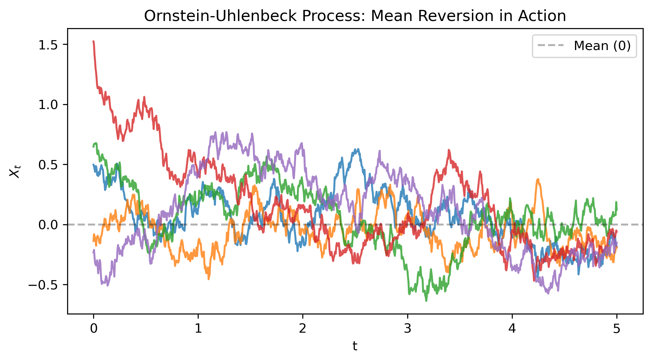Figure 3: Ornstein-Uhlenbeck process showing mean reversion. Paths are continuously pulled back toward zero.

Notice how the paths keep getting reverted back to zero. Unlike Brownian motion (Figure 1), which wanders off indefinitely, the OU process has a stationary distribution. We’ll derive the explicit solution once we cover Itô’s Lemma.

Itô’s Lemma

The main question is simple: if we have some function $f(X_t)$, how does it evolve when $X_t$ is stochastic? In regular calculus, we’d just use the chain rule: $df = f’(X) dX$.

In stochastic calculus, we get one extra term. For a process $X_t$ satisfying

and a smooth function $f(x, t)$, we start with a Taylor expansion

We truncate the Taylor series by keeping only terms of order $dt$. In ordinary calculus, all second-order terms like $(dt)^2$ are negligible. In stochastic calculus, some second-order terms are actually of order $dt$ and can’t be ignored. So we need to track which ones survive.

Start with $(dX_t)^2$. Substituting $dX_t = \mu \, dt + \sigma \, dW_t$ gives

Using the rules in Särkkä’s Applied Stochastic Differential Equations⁴ (Theorem 4.6):

• $(dt)^2 = 0$, a higher-order infinitesimal, so it vanishes
• $dt \cdot dW_t = 0$, also higher-order, so it vanishes
• $(dW_t)^2 = dt$, from equation (1) and the Quadratic Variation section

So $(dX_t)^2 = \sigma^2 \, dt$, which is not negligible.

The other second-order terms are

• $(dt)^2 = 0$
• $dt \cdot dX_t = dt \cdot (\mu \, dt + \sigma \, dW_t) = \mu(dt)^2 + \sigma \, dt \, dW_t = 0$

Only the $(dX_t)^2$ term remains. This gives us Itô’s Lemma

The last term, the Itô correction, comes from the roughness and quadratic variation of Brownian motion.

Expanding everything out by substituting the differential results into

So Itô’s Lemma is basically Taylor expansion for stochastic processes, keeping everything of order $dt$, including the important second-order term from $(dW_t)^2 = dt$.

Geometric Brownian Motion

With Itô’s Lemma in hand, we can solve geometric Brownian motion

where $\mu\in \mathbb{R}, ~ \sigma>0$. Here both the drift and diffusion depend on the state (unlike before). This falls into the family of linear multiplicative noise processes because the SDE is linear in $X_t$, but the “noise term” $dW_t$ multiplies $X_t$. (See Gardiner’s Handbook of Stochastic Methods³ Chapter 4.4.2 or Särkkä’s Applied Stochastic Differential Equations⁴ Example 4.6)

Set $Y_t = \log X_t$. We’ll apply Itô’s Lemma (equation 5) with $f(X, t) = \log X$ and work through the derivation step by step.

Step 1: Compute the partial derivatives. For $f(X, t) = \log X$:

• $\frac{\partial f}{\partial t} = 0$ (no explicit time dependence)
• $\frac{\partial f}{\partial X} = \frac{1}{X}$
• $\frac{\partial^2 f}{\partial X^2} = -\frac{1}{X^2}$

Step 2: Apply Itô’s Lemma. Using equation (5) with $\mu(X_t, t) = \mu X_t$ and $\sigma(X_t, t) = \sigma X_t$:

Substituting the derivatives:

Step 3: Substitute the original SDE. From equation (7), we have $dX_t = \mu X_t \, dt + \sigma X_t \, dW_t$. Substituting:

Now $dY_t$ no longer depends on the state. We’ve turned it into something we can integrate directly.

The Itô correction. See that $-\frac{\sigma^2}{2}$ term? That’s entirely from the second-order derivative in Itô’s Lemma. Without it, we’d get the wrong answer. This is a fundamental difference from ODEs: the nonlinearity of the logarithm interacts with the noise to create an extra drift term that wouldn’t exist in deterministic calculus.

At this point, the right-hand side is much simpler and can be solved with the tools from the Stochastic Integrals section.

Step 4: Integrate both sides (write the solution as integral form). Now we integrate both sides from $0$ to $t$:

The left side gives $Y_t - Y_0$ by the fundamental theorem of calculus.

The first integral on the right is ordinary: $\int_0^t \left( \mu - \frac{\sigma^2}{2} \right) ds = \left( \mu - \frac{\sigma^2}{2} \right) t$.

The second is a stochastic integral: $\sigma \int_0^t dW_s = \sigma (W_t - W_0) = \sigma W_t$ (since $W_0 = 0$).

Therefore

Step 5: Solve for $Y_t$. Rearranging terms gives

Since $Y_t=\log(X_t)$, we can resubstitute as

and exponentiating both sides gives us the solution to the SDE in equation (7)

Solving the Ornstein-Uhlenbeck Process

Now return to the OU process (equation 4) and derive its explicit solution. Recall the OU SDE

This is a linear SDE, and we can solve it using the integrating factor trick from ODEs. The goal is to find a transformation that eliminates the drift term so the transformed SDE has only additive noise, that is, a state-independent diffusion term scaled by Brownian motion $dW_t$.

Step 1: Choose the transformation. Consider $Y_t = X_t e^{\theta t}$, so $f(X, t) = X e^{\theta t}$. We’ll apply Itô’s Lemma to find $dY_t$.

Step 2: Compute the partial derivatives. For $f(X, t) = X e^{\theta t}$:

• $\frac{\partial f}{\partial t} = X \theta e^{\theta t} = \theta X e^{\theta t}$ (notice here $f$ has time dependency compared to the geometric Brownian motion earlier)
• $\frac{\partial f}{\partial X} = e^{\theta t}$
• $\frac{\partial^2 f}{\partial X^2} = 0$ (since $f$ is linear in $X$)

Step 3: Apply Itô’s Lemma. Using equation (5) with $\mu(X_t, t) = -\theta X_t$ and $\sigma(X_t, t) = \sigma$ to derive $dY_t$.

Substituting the derivatives:

Step 4: Substitute the original SDE. From the OU process, $dX_t = -\theta X_t \, dt + \sigma \, dW_t$. Substituting:

The drift terms cancel, so this gives

As before, we’ve transformed it into a state-independent SDE, so we can integrate it directly.

Step 5: Integrate both sides (write the solution as integral form). Integrating from $0$ to $t$:

Step 6: Substitute back and solve for $X_t$. Since $Y_t = X_t e^{\theta t}$ and $Y_0 = X_0 e^{\theta \cdot 0} = X_0$:

Multiplying both sides by $e^{-\theta t}$:

Using the property $e^{-\theta t} e^{\theta s} = e^{-\theta(t-s)}$, we write the final solution to the OU-process as

The first term is deterministic decay from the initial condition $X_0$. The second term is a stochastic integral where noise at each time $s$ is weighted by $e^{-\theta(t-s)}$, where recent noise contributes more than older noise.

Evaluating the stochastic integral: We can’t simplify $\int_0^t e^{-\theta(t-s)} dW_s$ further in closed form, but we can compute its statistical properties using the Itô isometry (equation 2).

Mean (expectation): Taking the expectation of equation (9):

The stochastic integral has zero mean (as we showed earlier), so the expected value decays exponentially to zero.

Variance: The stochastic integral is Gaussian with mean zero. Using Itô isometry (equation 2) with $g(s) = e^{-\theta(t-s)}$, we compute the variance:

Rewriting $e^{-2\theta(t-s)} = e^{-2\theta t} e^{2\theta s}$ and pulling out the constant to compute the ordinary integral:

So the total variance is:

Stationary distribution: As $t \to \infty$, the mean decays to zero ($\mathbb{E}[X_t] \to 0$) and the variance approaches $\sigma^2/2\theta$. Thus $X_\infty \sim \mathcal{N}(0, \sigma^2/2\theta)$. See Gardiner’s Handbook of Stochastic Methods (Section 4.4) for more details.

The Multidimensional Case

Everything we’ve done extends naturally to vector-valued processes. Consider $\mathbf{X}_t \in \mathbb{R}^n$ evolving as

where $\boldsymbol{\mu}: \mathbb{R}^n \times \mathbb{R} \to \mathbb{R}^n$ is the drift vector, $\boldsymbol{\Sigma}: \mathbb{R}^n \times \mathbb{R} \to \mathbb{R}^{n \times m}$ is the diffusion matrix, and $\mathbf{W}_t \in \mathbb{R}^m$ is an $m$-dimensional Brownian motion (with independent components).

For a scalar function $f(\mathbf{x}, t): \mathbb{R}^n \times \mathbb{R} \to \mathbb{R}$, Itô’s Lemma generalizes to:

Each term has a clear interpretation:

• $\frac{\partial f}{\partial t} dt$: explicit time dependence (same as 1D)

• \(\nabla f \cdot d\mathbf{X}_t = \sum_{i=1}^n \frac{\partial f}{\partial x_i} dX_i\): first-order change using the gradient $\nabla f = \left(\frac{\partial f}{\partial x_1}, \ldots, \frac{\partial f}{\partial x_n}\right)$

• $\frac{1}{2} \sum_{i,j} \frac{\partial^2 f}{\partial x_i \partial x_j} (\boldsymbol{\Sigma} \boldsymbol{\Sigma}^\top)_{ij} \, dt$: Itô correction using the Hessian matrix of second derivatives

The key difference from 1D is that the Itô correction now involves $\boldsymbol{\Sigma} \boldsymbol{\Sigma}^\top$, the covariance matrix of the noise. This comes from $(dX_i)(dX_j) = (\boldsymbol{\Sigma} \boldsymbol{\Sigma}^\top)_{ij} \, dt$, the multidimensional version of $(dW_t)^2 = dt$.
For more detail, see Särkkä’s Applied Stochastic Differential Equations⁴ Theorem 4.2 for a practical derivation of Itô’s Lemma.

A 2-Dimensional Problem: Brownian Motion on a Circle

To put the pieces together, consider a geometric example: Brownian motion on a circle. This makes it easier to see how Itô’s Lemma handles curved spaces and why the correction term matters geometrically.

Setup

Consider a point moving on the unit circle in $\mathbb{R}^2$. We can parameterize the position as

where $\theta_t$ is the angle at time $t$. Although the state space is 2-dimensional, the system is effectively 1-dimensional since it’s completely determined by the angle $\theta$.

We let the angle evolve through changes induced by Brownian motion via

This means the point performs a random walk along the circle, moving clockwise or counterclockwise based on the Brownian increments as shown in the Figure below.

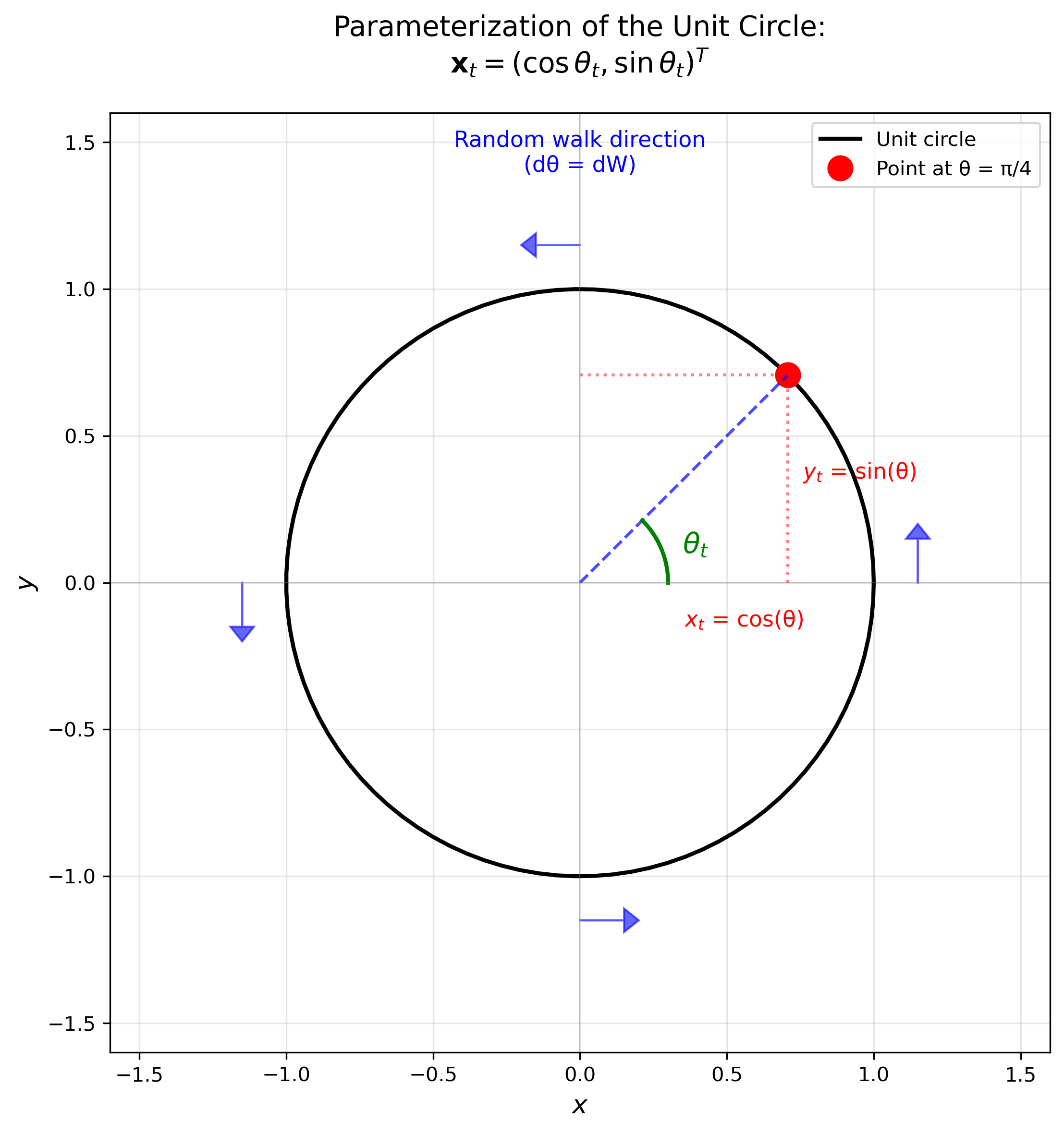
Figure: Parameterization of the unit circle using the angle $\theta_t$. The position $\mathbf{x}_t = (\cos\theta_t, \sin\theta_t)$ is completely determined by the angle, which evolves randomly via $d\theta_t = dW_t$. Blue arrows indicate the direction of the random walk.

Applying Itô’s Lemma

The next question is what SDEs the Cartesian coordinates $x_t = \cos \theta_t$ and $y_t = \sin \theta_t$ satisfy. We’ll apply Itô’s Lemma to each component. The random fluctuations are in $\theta$, and Itô’s Lemma tells us how they propagate to $(x, y)$.

Step 1: Compute the partial derivatives for $x_t = \cos \theta_t$. For $f(\theta, t) = \cos \theta$:

• $\frac{\partial f}{\partial t} = 0$ (no explicit time dependence)
• $\frac{\partial f}{\partial \theta} = -\sin \theta$
• $\frac{\partial^2 f}{\partial \theta^2} = -\cos \theta$

Step 2: Apply Itô’s Lemma to find $dx_t$. Using equation (5) with $\mu(\theta_t, t) = 0$ and $\sigma(\theta_t, t) = 1$ (since $d\theta_t = dW_t$):

Substituting the derivatives:

Step 3: Compute the partial derivatives for $y_t = \sin \theta_t$. For $g(\theta, t) = \sin \theta$:

• $\frac{\partial g}{\partial t} = 0$ (no explicit time dependence)
• $\frac{\partial g}{\partial \theta} = \cos \theta$
• $\frac{\partial^2 g}{\partial \theta^2} = -\sin \theta$

Step 4: Apply Itô’s Lemma to find $dy_t$. Similarly, using equation (5):

Substituting the derivatives:

Substituting $x_t = \cos \theta_t$ and $y_t = \sin \theta_t$, we get the vector SDE

Geometric Interpretation

Look at what’s happening geometrically:

The diffusion term $(-y_t, x_t)^T dW_t$ is orthogonal to the position vector $(x_t, y_t)^T$. It points along the tangent direction of the circle and moves the point along its boundary.

The drift term $-\frac{1}{2}(x_t, y_t)^T dt$ points toward the origin. It compensates for the second-order effect of the stochastic motion and keeps the process on the circle in continuous time.

Together, these terms produce Brownian motion in the angular direction while preserving the circular constraint. The drift continuously projects the position back onto the manifold, counteracting the curvature effects from the nonlinear transformation $\theta \to (x, y)$.

Simulation: Exact vs. Numerical Methods

We can verify this by comparing two simulations.

Method 1: Angular simulation (exact). We directly simulate $d\theta_t = dW_t$ and convert to Cartesian coordinates $(x_t, y_t) = (\cos \theta_t, \sin \theta_t)$. This stays exactly on the circle by construction.

Method 2: Euler-Maruyama on the 2D SDE (numerical approximation). We discretize the Cartesian SDE using the Euler-Maruyama scheme

This numerical scheme has discretization error. It doesn’t keep the point exactly on the circle. The drift only approximates the continuous projection onto the manifold.

import numpy as np
import matplotlib.pyplot as plt

np.random.seed(42)
T = 5.0
n_steps = 1000
n_paths = 5
dt = T / n_steps
t = np.linspace(0, T, n_steps + 1)

# Method 1: Simulate angular BM (stays exactly on circle)
theta_exact = np.zeros((n_paths, n_steps + 1))
theta_exact[:, 0] = np.random.uniform(0, 2*np.pi, n_paths)
for i in range(n_steps):
    dW = np.sqrt(dt) * np.random.randn(n_paths)
    theta_exact[:, i+1] = theta_exact[:, i] + dW

x_exact = np.cos(theta_exact)
y_exact = np.sin(theta_exact)

# Method 2: Euler-Maruyama on the 2D SDE (has discretization error)
np.random.seed(42)  # Same random numbers for fair comparison
x_em = np.zeros((n_paths, n_steps + 1))
y_em = np.zeros((n_paths, n_steps + 1))
x_em[:, 0] = np.cos(theta_exact[:, 0])
y_em[:, 0] = np.sin(theta_exact[:, 0])

for i in range(n_steps):
    dW = np.sqrt(dt) * np.random.randn(n_paths)
    # Euler-Maruyama step
    x_em[:, i+1] = x_em[:, i] - 0.5 * x_em[:, i] * dt - y_em[:, i] * dW
    y_em[:, i+1] = y_em[:, i] - 0.5 * y_em[:, i] * dt + x_em[:, i] * dW

# Compute radii
radii_exact = np.sqrt(x_exact**2 + y_exact**2)
radii_em = np.sqrt(x_em**2 + y_em**2)

# Create visualization
fig = plt.figure(figsize=(14, 10))
gs = fig.add_gridspec(2, 2, height_ratios=[1, 1])
ax1 = fig.add_subplot(gs[0, 0])
ax2 = fig.add_subplot(gs[0, 1])
ax3 = fig.add_subplot(gs[1, :])

colors = plt.cm.viridis(np.linspace(0, 1, n_paths))

# Plot 1: Exact method
circle1 = plt.Circle((0, 0), 1, color='lightgray', fill=False, linewidth=2)
ax1.add_patch(circle1)
for i in range(n_paths):
    ax1.plot(x_exact[i], y_exact[i], alpha=0.7, linewidth=1.5, color=colors[i])
    ax1.plot(x_exact[i, 0], y_exact[i, 0], 'o', markersize=8, color=colors[i])
ax1.set_xlim(-1.5, 1.5); ax1.set_ylim(-1.5, 1.5)
ax1.set_aspect('equal'); ax1.grid(alpha=0.3)
ax1.set_xlabel('$x_t$'); ax1.set_ylabel('$y_t$')
ax1.set_title('Method 1: Angular Simulation (Exact on Circle)')

# Plot 2: Euler-Maruyama
circle2 = plt.Circle((0, 0), 1, color='lightgray', fill=False, linewidth=2)
ax2.add_patch(circle2)
for i in range(n_paths):
    ax2.plot(x_em[i], y_em[i], alpha=0.7, linewidth=1.5, color=colors[i])
    ax2.plot(x_em[i, 0], y_em[i, 0], 'o', markersize=8, color=colors[i])
ax2.set_xlim(-1.5, 1.5); ax2.set_ylim(-1.5, 1.5)
ax2.set_aspect('equal'); ax2.grid(alpha=0.3)
ax2.set_xlabel('$x_t$'); ax2.set_ylabel('$y_t$')
ax2.set_title('Method 2: Euler-Maruyama on 2D SDE (Discretization Error)')

# Plot 3: Radius over time
for i in range(n_paths):
    ax3.plot(t, radii_exact[i], alpha=0.7, linewidth=1.5, 
             color=colors[i], linestyle='-')
    ax3.plot(t, radii_em[i], alpha=0.7, linewidth=1.5, 
             color=colors[i], linestyle='--')
ax3.axhline(1, color='red', linestyle=':', linewidth=2, label='True radius')
ax3.set_xlabel('Time $t$'); ax3.set_ylabel('Radius $r_t$')
ax3.set_title('Radius Over Time: Exact (solid) vs Euler-Maruyama (dashed)')
ax3.legend(); ax3.grid(alpha=0.3)

plt.tight_layout()
plt.savefig("/Users/tuanle/Desktop/projects/tuanle618.github.io/assets/img/blogs/stochastic-calculus/brownian_circle.png",
            dpi=300, bbox_inches='tight')
plt.show()

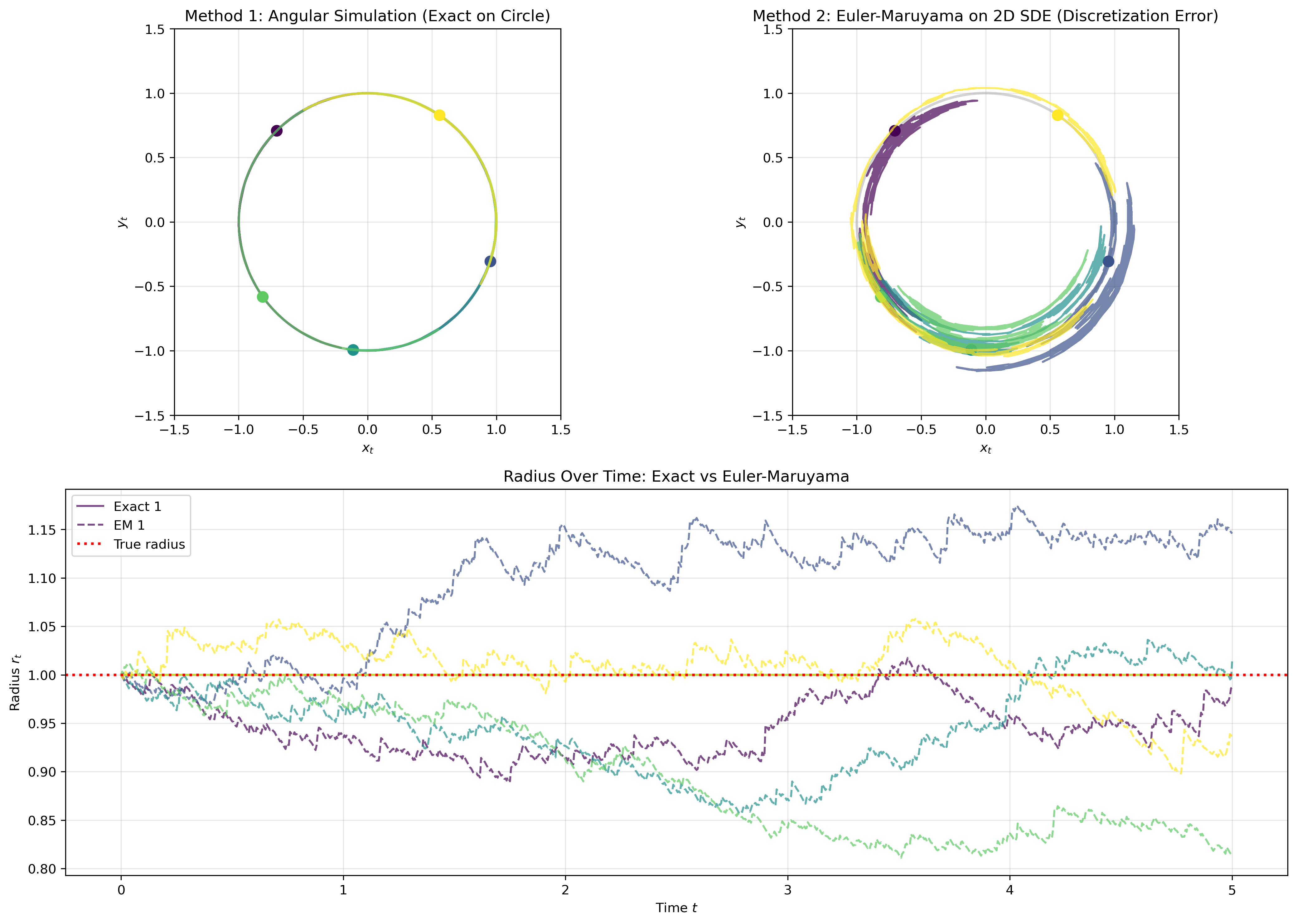Figure 4: Comparison of exact (angular) vs. approximate (Euler-Maruyama) methods for Brownian motion on a circle. Top: trajectories on the circle. Bottom: radius evolution showing discretization errors.

The exact angular method (left) stays perfectly on the circle, while Euler-Maruyama (right) drifts off slightly. You can see this in the bottom panel where the dashed lines deviate from radius 1.0. Working directly with the intrinsic coordinate $\theta$ gives exact results, but the Cartesian discretization has errors that accumulate over time.

One more way to read the diffusion term is through a Lie algebra matrix. Define

Then the infinitesimal rotation can be expressed as

The matrix $A_\theta$ is an element of $\mathfrak{so}(2)$, the Lie algebra of the rotation group $SO(2)$. This is the generator of infinitesimal rotations. The same perspective extends to Brownian motion on higher-dimensional manifolds, where the diffusion term is written as a Lie algebra element acting on the current position. That is one route into stochastic dynamics on Lie groups and their applications in diffusion models on manifolds. I’ll come back to that in the next blog post.

Conclusion

Stochastic calculus starts with one unusual fact: $(dW_t)^2 = dt$. From there you get stochastic integrals, Itô’s Lemma, and practical ways to solve SDEs such as geometric Brownian motion and the Ornstein-Uhlenbeck process. The recurring move is to find a transformation that turns a state-dependent equation into one you can integrate directly.

Brownian motion on a circle shows the same idea from a geometric angle. The Itô correction is not a minor detail. It is what keeps the transformed dynamics consistent with the space the process lives on, and it opens the door to stochastic dynamics on manifolds and Lie groups.

References